Name: Naïve Bayes
Category: Supervised prediction - classification
Introduction
Suppose you've just been handed a set of data by your boss that contains sales transactions for the last six months. There are quite a few fields in the data and a surprising number of transactions have occurred over that time period. You get told that losses due to credit card fraud are starting to hurt the business and something needs to be done about it. It would really help to be able to identify new transactions with a high chance of being fraudulent before the company ships out merchandise. Fortunately, the dataset contains a column that indicates, for each transaction, whether or not it involved fraudulent credit card usage. This means you can use machine learning classification algorithms to find the patterns in the data that relate to fraud. Unfortunately, your boss would like an indication of whether a solution to the problem is feasible by the end of the day. This means that there is no time to do the sort of data preparation and experimentation required for optimizing sophisticated learning algorithms. Panic sets in...
... and then subsides as you remember the Naïve Bayes algorithm. Naïve Bayes is the perfect choice, in this case, for a quick investigation because it can work directly with both categorical and numeric input columns, learns quickly even when there are lots of rows and columns in the data, and provides a good baseline to compare accuracy of more sophisticated methods. Naïve Bayes will, at the very least, show if there is some sort of relationship between the data collected about a transaction and whether it turned out to involve fraudulent credit card usage or not.
The Naïve Bayes Method
The naïve Bayes algorithm is a statistical method for building a model that can produce predictions for a categorical class attribute through a simple application of the Bayes' rule of conditional probability.
Bayes' rule states that if you have hypothesis H and evidence E (that bears on that hypothesis), then

In the supervised classification case, H are class labels and E are attribute/input values. So, the formula tells us that the chance (or likelihood to be precise) of each class label is proportional to the frequency (or, more correctly, probability) that attribute values occur within that class. Rather than computing the joint probability of the attribute value combinations in E, naïve Bayes is "naïve" simply because it makes the (gross) assumption that attribute values are independent of one another given the class value. If we make this assumption, then it is valid to simply multiply the individual attribute probabilities. Interestingly, while this independence assumption is almost always violated on real data, predictions produced by naïve Bayes are often quite accurate in practice. The reason for this is that the resulting probability estimates, while skewed by the independence assumption, often result in the highest likelihood being assigned to the actual class label.
Strengths
- Simple to implement
- Fast: scales linearly in the number of instances (rows) and attributes (columns)
- Often accurate despite the independence assumption
- Works well with categorical data and for multi-class problems
Weaknesses
- Independence assumption affects probability estimation which, in turn, can affect accuracy
- Low representational power
- Typical modeling of numeric attributes via Gaussian distributions might not be appropriate in all cases
Model interpretability: medium/low
Per-class parameters/counts for the attribute estimators are the typical output.
Common Uses
Naïve Bayes, due to its simplicity, is often used as a baseline algorithm against which to compare more powerful methods. Naïve Bayes is also what is commonly referred to as an anytime algorithm. In practical terms, this means that the internal statistics that comprise the naïve Bayes model can be updated incrementally (i.e., row-by-row) and it is able to produce a prediction at any point in time. When compared to most machine learning methods that require all the training data to be examined before predictions can be made, and combined with its low memory/processing requirements, naïve Bayes is an ideal choice for IoT applications running at the edge on low-cost hardware. One application that naïve Bayes has proven well suited for is that of text classification. In this case, the idea is to automatically assign a document to a pre-defined category based on the words that occur within it. The spam filter in your email client could quite easily be implemented using a naïve Bayes model. In this case there are only two categories of email: spam and ham. However, naïve Bayes' ability to handle multi-class problems means that you could easily train it to assign email into many different categories, such as "work-related", "personal", "mailing-list", and so on.
Configuration
In terms of settings to tweak, naïve Bayes couldn't be simpler.
If you use the implementation in MLlib, then there is basically nothing to configure! However, this implementation is limited to categorical input attributes only. So, if you have numeric columns in your data you will have to convert them to categorical via binning.
On the other hand, the implementation in Weka does handle numeric attributes and provides several settings you can experiment with. By default, this implementation models numeric attributes with Gaussian distributions. There is an option to replace this with kernel density estimation, and you can use this if you suspect that there are some attributes that don't follow a normal distribution within each class. However, be aware that fitting kernel density estimates is slower than fitting Gaussian distributions. Alternatively, the Weka implementation provides an option to bin numeric attributes automatically using an MDL-based supervised discretization technique.
Example
Let's consider a very simple dataset for learning our first naïve Bayes model. This dataset, involving a single denormalized table (see weather_nominal.xls), concerns the conditions that are suitable for playing some unspecified game. In general, instances (rows of the spreadsheet) in a dataset are characterized by the values of features, or attributes (columns of the spreadsheet), that measure different characteristics of the instance. The weather dataset is shown in the following screenshot:
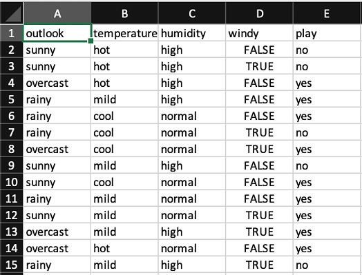
There are four attributes: outlook, temperature, humidity and windy. The outcome is whether to play or not. All four attributes have values that are symbolic categories rather than numbers. For example, outlook can be sunny, overcast, or rainy. Two of the attributes have three distinct values each, and the other two attributes have two distinct values. This gives a total of 36 possible combinations, of which 14 are present in the dataset.
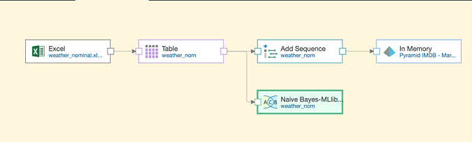
Now let's load this dataset into Pyramid and take a look at the distribution of the class value by various attribute combinations. We can build a new data model based on the weather data in the ETL application like so:
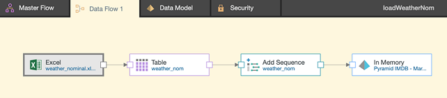
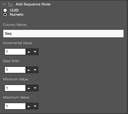
In this case, we've used the Add Sequence node to add a constant value of 1 to each row in the data. We can use this as a measure in the Discovery application when exploring the data. We've configured Add Sequence as shown below:
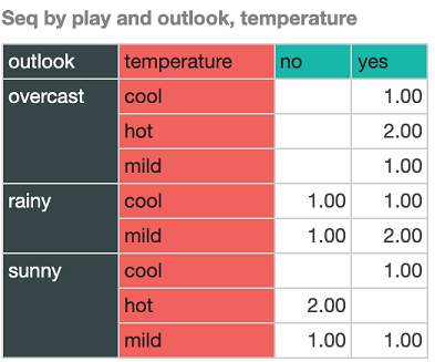
Here we can see counts of the play outcome broken down by outlook and temperature. Note that empty cells indicate that we haven't got an example of that particular combination of outlook and temperature values in our dataset. Things are pretty clear cut when it's overcast - temperature (and the other two attributes) have no bearing, and we always play. It's a mixed bag when it's rainy. In this case, there is a preference to play, but only when temperature is mild. When it's sunny, there is evidence to suggest that we will play when temperature is cool, stronger evidence to suggest that we won't when it's hot, and it could go either way when the temperature is mild.
Now we can build a naïve Bayes model to predict the outcome for a new day by training it the weather data. The easiest way to do this is to simply add the Naïve Bayes-MLlib node to our existing data flow, as shown below:
And then we configure it like so:
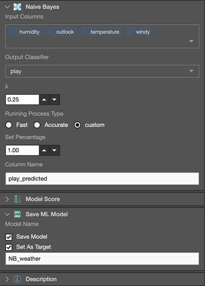
Here we can see that we've selected humidity, outlook, temperature and windy as inputs to naïve Bayes; and play has been selected as the output (i.e., class attribute to predict). Because this is a very small dataset, under Running Process Type we've opted to use all the data to train on. The output will include an additional column containing the predicted class label which, in this case, we've opted to call "play_predicted." Finally, we've chosen to save the naïve Bayes to a file called "NB_weather" so that it can be used in the future to predict on a given day whether it would be suitable for playing or not.
Previewing the output of the naïve Bayes node produces this table:
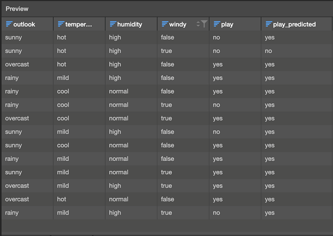
Our classifier makes four incorrect predictions on the data. You can start to understand why the model makes certain mistakes by returning to the Discovery app to look at the frequency of certain attribute-class value combinations. In the Preview table above, we can see that the model actually only predicts play=no in one case (the second row). This isn't too surprising because we have 9 examples of play=yes and only 5 of play=no in our training data, so, the prior evidence supports playing the game right from the outset (in the absence of any other information). The first and second rows of the table are quite interesting because they are both examples of play=no, and they differ only in the value of windy. Our model gets the first one wrong and the second one correct. Given that naïve Bayes treats attributes independent of one another given the class, we can get a feeling for what is happening by looking at the counts for windy:
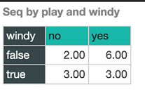
When windy is false, as it is in the first example, the 6/9 evidence that contributes for play=yes versus the 2/5 evidence it contributes for play=no is enough to result in yes being the most likely class value. However, in the case of windy=true, the counts are split evenly between play=yes and play=no which, in-turn, provides more weight for no - that is, 3/5 versus 3/9. This is enough support for no to make it the most likely class value.
You might be wondering what happens when a value for a given attribute never occurs in conjunction with one of the class values in the training data. In this case, we would have a count of zero and a corresponding probability of zero for that combination. This, in turn, would veto the evidence contributed by the other attribute values for that class value when the probabilities are multiplied, resulting in an overall probability of zero. This is referred to as the zero frequency problem. In this case, there is a simple solution that works well in practice. Instead of starting counts from zero when learning the model, we can start with a small non-zero value. This initial count is the parameter shown in the screenshot where we configured the model. The default provided is 0.25, but any small value can be used (a value of 1 is another common choice).